Plotting things
SMURFS implements quite a lot of different plotting mechanisms. So lets have a look at the different ways you can plot things with SMURFS. Lets first get some data and analyze it:
[1]:
from smurfs import Smurfs
[2]:
star = Smurfs(target_name='Gamma Doradus')
 Searching processed light curves for Gamma Doradus on mission(s) TESS ...
 Resolving Gamma Doradus to TIC using MAST ...
 TIC ID for Gamma Doradus: TIC 219234987
 Short cadence observations available for Gamma Doradus. Downloading ...
Warning: 31% (6168/19692) of the cadences will be ignored due to the quality mask (quality_bitmask=175).
 Found processed light curve for Gamma Doradus!
 Using TESS observations! Combining sectors ...
 Total observation length: 78.32 days.
 Duty cycle for Gamma Doradus: 84.45%
[3]:
star.run(snr=4,window_size=2)
 Periodogramm from 0.0 1 / d to 360.0 1 / d
 Starting frequency extraction.
 Skip similar:  Deactivated
 Chancel after 10 similar:  Activated
 Window size: 2
 Number of extended frequencies: 0
 Nyquist frequency: 360.0 1 / d
 List of frequencies, amplitudes, phases, S/N
 F0   1.363601+/-0.000004 1 / d   0.01056+/-0.00008 mag   0.5105+/-0.0011   14.621917538996478
 F1   1.3214676+/-0.0000031 1 / d   0.01011+/-0.00006 mag   0.8538+/-0.0009   17.646618113213755
 F2   1.470851+/-0.000007 1 / d   0.002806+/-0.000035 mag   0.8600+/-0.0020   7.578344472336695
 F3   1.878144+/-0.000007 1 / d   0.002413+/-0.000032 mag   0.5167+/-0.0021   6.717143847007492
 F4   1.385307+/-0.000007 1 / d   0.002228+/-0.000030 mag   0.1748+/-0.0022   7.318522855378772
 F5   0.316642+/-0.000008 1 / d   0.002030+/-0.000028 mag   0.2544+/-0.0022   5.597834999218046
 F6   1.417226+/-0.000008 1 / d   0.001813+/-0.000027 mag   0.3842+/-0.0024   6.523381016995975
 F7   2.742524+/-0.000008 1 / d   0.001779+/-0.000026 mag   0.9427+/-0.0023   9.558566515908968
 F8   0.112357+/-0.000008 1 / d   0.001629+/-0.000024 mag   0.0235+/-0.0024   5.27044577952894
 F9   1.237200+/-0.000009 1 / d   0.001393+/-0.000023 mag   0.0913+/-0.0026   5.176607940138036
 F10   1.681520+/-0.000011 1 / d   0.001115+/-0.000022 mag   0.1662+/-0.0032   4.585937811798608
 Stopping extraction after 11 frequencies.
 Total frequencies: 11
 Gamma Doradus Analysis done!
Plotting the light curve
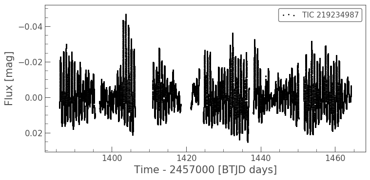
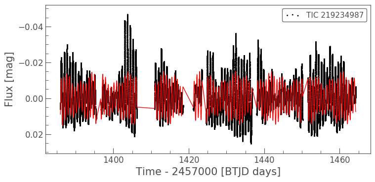
Now, if you want to plot the light curve, you can call the plot_lc method
[4]:
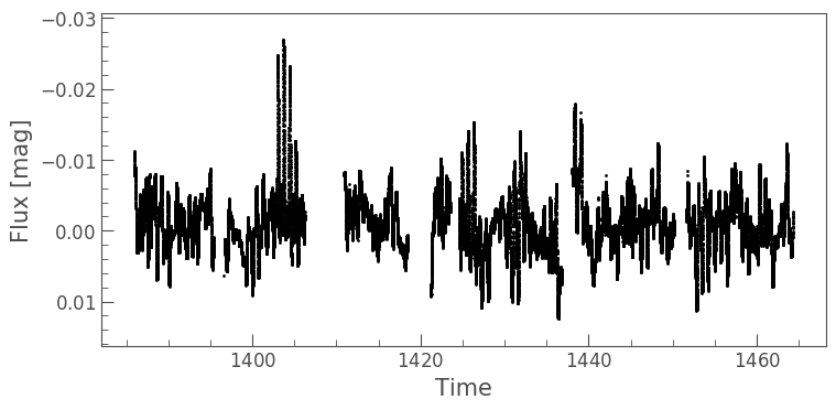
star.plot_lc()

In black you can see the data set, in red the model.
In the backend, SMURFS uses the lightkurve.LightCurve.plot method to plot the light curve. You have access to all the parameters for these objects. We can make use of this if we want to plot the light curve without the model:
[5]:
star.lc.scatter()
[5]:
<matplotlib.axes._subplots.AxesSubplot at 0x1319cb5c0>
Plotting periodograms
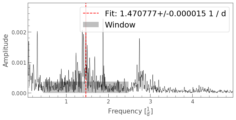
What is true for the LightCurve objects, is also true for the periodogram. To plot the periodogram, including the significant frequencies, you can use the plot_pdg function
[6]:
star.plot_pdg()
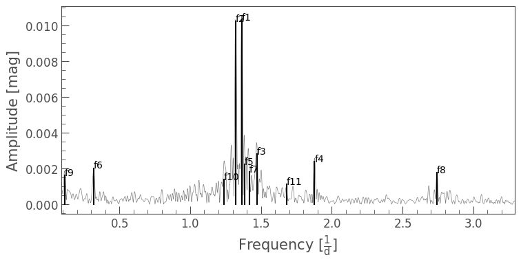
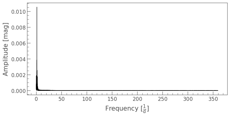
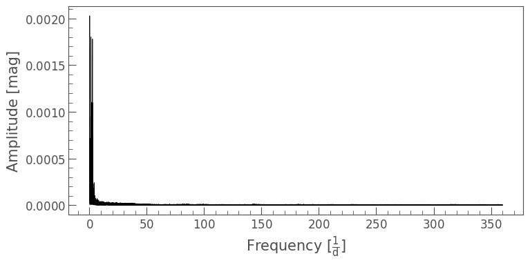
This of course restricts us to the range where significant frequencies have been found. If we want the whole periodogram, we can use the pdg property
[7]:
star.pdg.plot()
[7]:
<matplotlib.axes._subplots.AxesSubplot at 0x13246d518>
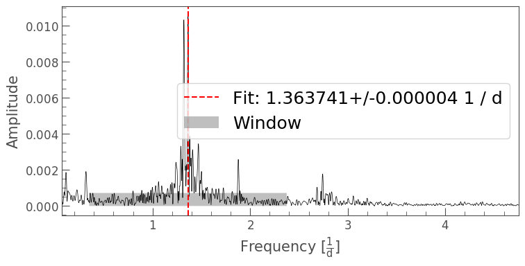
The individual frequencies
As noted in previous chapters, the result property also contains all the individual frequencies. You can access them using iloc
[8]:
star.result
[8]:
| f_obj | frequency | amp | phase | snr | res_noise | significant | |
|---|---|---|---|---|---|---|---|
| 0 | <smurfs._smurfs.frequency_finder.Frequency obj... | 1.363741+/-0.000004 | 0.01033+/-0.00008 | 0.3267+/-0.0012 | 14.621918 | -0.000890 | True |
| 1 | <smurfs._smurfs.frequency_finder.Frequency obj... | 1.321203+/-0.000004 | 0.01025+/-0.00008 | 1.2294+/-0.0012 | 17.646618 | -0.000841 | True |
| 2 | <smurfs._smurfs.frequency_finder.Frequency obj... | 1.470777+/-0.000015 | 0.00281+/-0.00008 | 0.965+/-0.004 | 7.578344 | -0.000855 | True |
| 3 | <smurfs._smurfs.frequency_finder.Frequency obj... | 1.878144+/-0.000017 | 0.00241+/-0.00008 | 0.517+/-0.005 | 6.717144 | -0.000854 | True |
| 4 | <smurfs._smurfs.frequency_finder.Frequency obj... | 1.385307+/-0.000018 | 0.00223+/-0.00008 | 0.175+/-0.005 | 7.318523 | -0.000865 | True |
| 5 | <smurfs._smurfs.frequency_finder.Frequency obj... | 0.316642+/-0.000020 | 0.00203+/-0.00008 | 0.254+/-0.006 | 5.597835 | -0.000865 | True |
| 6 | <smurfs._smurfs.frequency_finder.Frequency obj... | 1.417226+/-0.000023 | 0.00181+/-0.00008 | 0.384+/-0.007 | 6.523381 | -0.000859 | True |
| 7 | <smurfs._smurfs.frequency_finder.Frequency obj... | 2.742524+/-0.000023 | 0.00178+/-0.00008 | 0.943+/-0.007 | 9.558567 | -0.000859 | True |
| 8 | <smurfs._smurfs.frequency_finder.Frequency obj... | 0.112357+/-0.000025 | 0.00163+/-0.00008 | 0.023+/-0.007 | 5.270446 | -0.000856 | True |
| 9 | <smurfs._smurfs.frequency_finder.Frequency obj... | 1.237200+/-0.000029 | 0.00139+/-0.00008 | 0.091+/-0.009 | 5.176608 | -0.000856 | True |
| 10 | <smurfs._smurfs.frequency_finder.Frequency obj... | 1.68152+/-0.00004 | 0.00112+/-0.00008 | 0.166+/-0.011 | 4.585938 | -0.000860 | True |
[9]:
star.result.iloc[5].f_obj.plot()
[9]:
<matplotlib.axes._subplots.AxesSubplot at 0x136cbfba8>
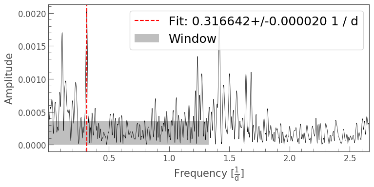
To plot the corresponding light curve, we can access them through the corresponding property
[10]:
star.result.iloc[5].f_obj.lc.scatter()
[10]:
<matplotlib.axes._subplots.AxesSubplot at 0x136cec278>
We can also take a look at the whole periodogram
[11]:
star.result.iloc[5].f_obj.pdg.plot()
[11]:
<matplotlib.axes._subplots.AxesSubplot at 0x130aaf6a0>
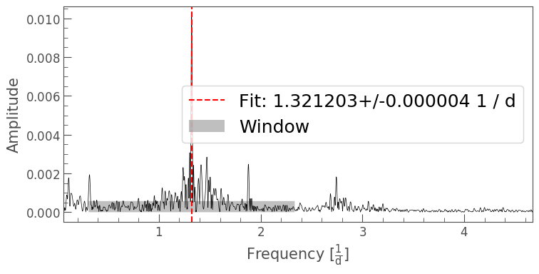
We can also plot as many as we like here. For example the first three:
[12]:
star.result.iloc[0].f_obj.plot()
star.result.iloc[1].f_obj.plot()
star.result.iloc[2].f_obj.plot()
[12]:
<matplotlib.axes._subplots.AxesSubplot at 0x12fe0d550>
Plotting only part of the model
We might also be interested to only plot part of the model. For this, we copy the result from the smurfs object and restrict ourselves to the interesting frequencies:
[14]:
model = star.result.iloc[[0,2,5]]
[15]:
model
[15]:
| f_obj | frequency | amp | phase | snr | res_noise | significant | |
|---|---|---|---|---|---|---|---|
| 0 | <smurfs._smurfs.frequency_finder.Frequency obj... | 1.363741+/-0.000004 | 0.01033+/-0.00008 | 0.3267+/-0.0012 | 14.621918 | -0.000890 | True |
| 2 | <smurfs._smurfs.frequency_finder.Frequency obj... | 1.470777+/-0.000015 | 0.00281+/-0.00008 | 0.965+/-0.004 | 7.578344 | -0.000855 | True |
| 5 | <smurfs._smurfs.frequency_finder.Frequency obj... | 0.316642+/-0.000020 | 0.00203+/-0.00008 | 0.254+/-0.006 | 5.597835 | -0.000865 | True |
[18]:
star.plot_lc(result=model)
[19]:
star.plot_lc()
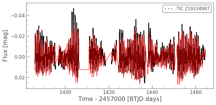
You can of course use any filtering you like with pandas.
[ ]: